Attaching package: 'igraph'The following objects are masked from 'package:stats':
decompose, spectrumThe following object is masked from 'package:base':
union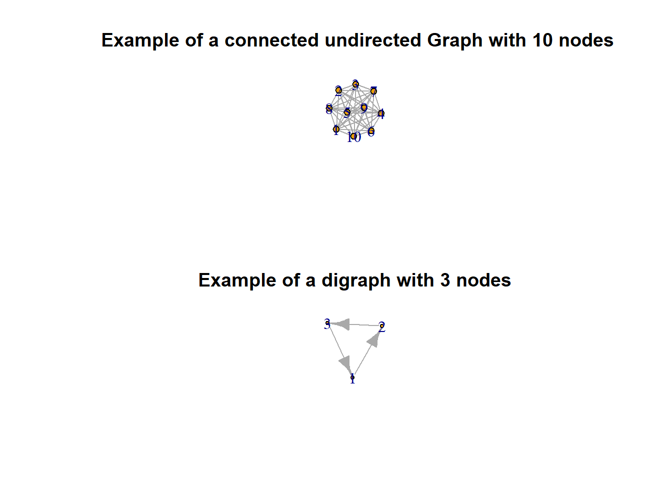
The \(21^{st}\) Century was marked by the advent of the digital age. Now, our world is more connected sand data driven than ever before. Some of the questions of interest are as follows :
1. How many people, on an average are mutual connections between two people on Facebook?
2. Can we identify different communities in a society ?
3. How well connected are my friends among themselves ?
4. How influential is a person in this society ?
These and many more can be answered via network data analysis (NDA). NDA primarily stands on the foundations of graph theory and data analysis environmetns/languages.
The study of graphs began in \(18^{th}\) century after Euler solved the Konigsberg problem. The German city of Königsberg (present-day Kaliningrad, Russia) is situated on the Pregolya river. The geographical layout is composed of four main bodies of land connected by a total of seven bridges.The problem was as follows :
“Was it possible to take a walk through the town in such a way as to cross over every bridge once, and only once?”
Euler showed that it is not possible by applying what we now call graph theory. Since then, graphs have been studied extensively. Here we present some definitions which we shall need later.
1. Graph : It is an ordered pair \[(V,E)\] where \(V\) denotes the (finite) set of nodes or vertices and E denotes the set of edges.Edges are unordered pairs of vertices.An edge that joins itself is called a loop. A graph without a loop is called a simple graph.
2. Directed Graph : If we consider ordered pairs in place of unordered pairs the resultant graph is called directed graph. We note that if a graph is not directed it is called undirected. It is also called digraph.
3. Multi Graph : A graph for which we have more than one edge between same nodes.
4. Complete Graph : A graph is called complete if it contains all possible edges.
5. Connected Graph : A graph is called connected if there exists a path between any two vertices.
6. Subgraph : Suppose we have a graph \(\Gamma=(V,E)\). Then \(S=(V_{1},E_{1})\) is called a subgraph of \(\Gamma\) iff \(V_{1}\subseteq\) \(V\) and \(E_{1}\subseteq\) \(E\).
7. Induced Subgraph : Suppose we have a graph \(\Gamma=(V,E)\). Then \(S=(V_{1},E_{1})\) is called an induced subgraph of \(\Gamma\) if \(V_{1}\subseteq\) \(V\) and the edge contains all the edges with end points in \(V_{1}\) and contained in \(\Gamma\).
8. Adjacency Matrix : Adjacency matrix of a graph embedds the information regarding the edges and weights of a graph ( directed or undirected ). The \((i,j)^{th}\) element is 0, if there is no node. For an unweighted digraph the \((i,j)^{th}\) element is 1 if there is an edge from i to j. For a weighted graph , 1 is replaced by the respective weight. We note that if the graph is undirected the adjacency matrix is symmetric. Some illustration with R is as follows :
Attaching package: 'igraph'The following objects are masked from 'package:stats':
decompose, spectrumThe following object is masked from 'package:base':
union
Data analysis of Network Data can be performed in both R and Python. R has some great user-friendly packages, the most prominent of which is \(igraph\). This package has functions to take network data as input, to generate random graphs of various types ( Erdos-Renyi, Small-World,etc) , visualize networks and contains at least 12 inbuilt packages ( collected from various sources ). However, we note that R cannot handle large data sets properly. As most real world network data contain thousands ( and sometimes millions) of nodes, it is advised to analyse large datasets in Python. For Python ,SNAP ( Stanford Network Analysis Project ) have developed snap.py which can be used for network analysis in Python. However, we note that this does not run on new versions of R. It runs on R 3.7. Versions 3.7.2 and 3.7.6 are not compatible, but version 3.7.8 has been claimed to work. Finally, some good sources for network datasets are as follows :
SNAP ( Stanford Network Analysis Project )
UCI Network Data Repository
Duke Data Analysis Center
Just like in classical statistics, we need descriptive measures to understand the data well, as well as new measures to understand and study various topological properties inherent in real life data sets. For networks the following ideas are foundation in nature :
Vertex Centrality : Vertex Centrality quantifies how ``central’’ or important some nodes are in the network.
Network Cohesion : It is in our interest to measure to what extent the nodes in the dataset are cohesive.
Community Detection : It may be our interest to identify subgraphs which tend to be more identical in some manner such that the nodes can be grouped into \(communities\). These \(communities\) can be disjoint or intrinsic ( one embedded into the other) or overlapping.
Now, we define popular measures to quantify the above mentioned notions
in real world graphs.
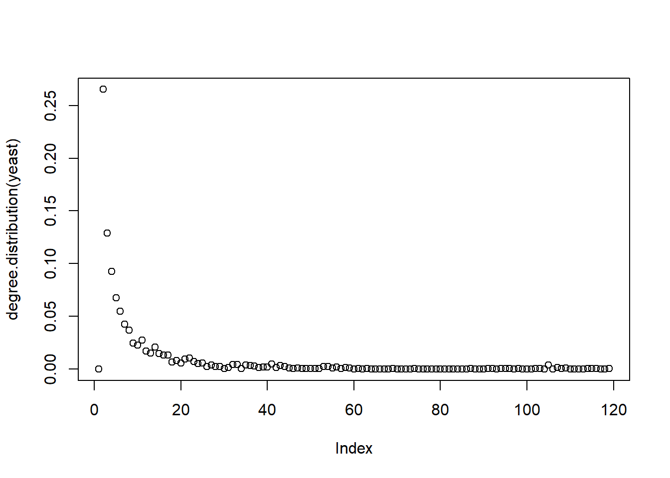
Degree Centrality : \(C_{i}=d(w_{i})\) where \(w_{i}\)is the \(i^{th}\)node.
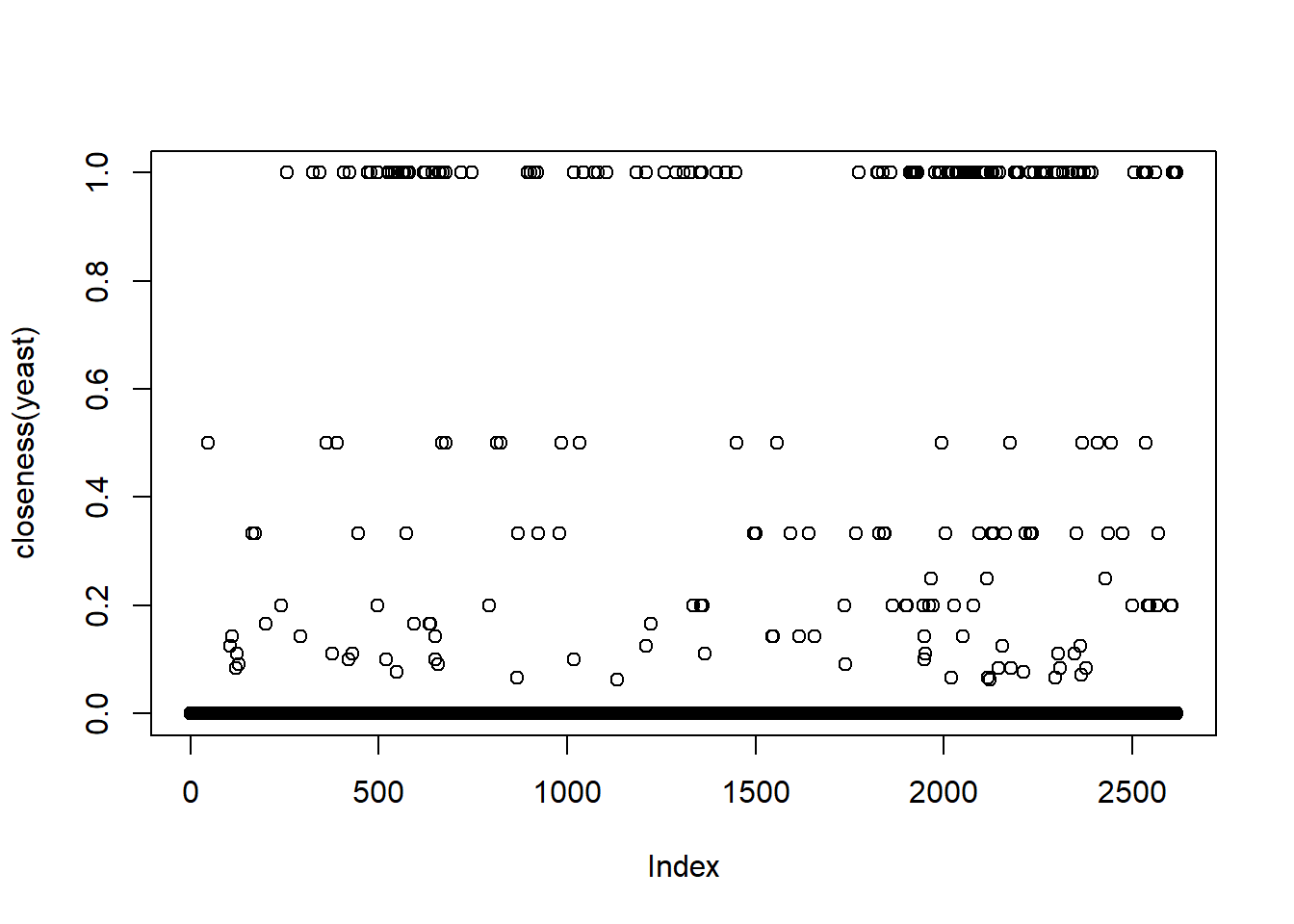
Closeness Centrality : \(C_{i}=\frac{n-1}{\sum_{j=1,j\nshortparallel i}^{n-1}d(w_{i},w_{j})}\). This is the reciprocal of sum of all distances of \(i^{th}node\) to other nodes.
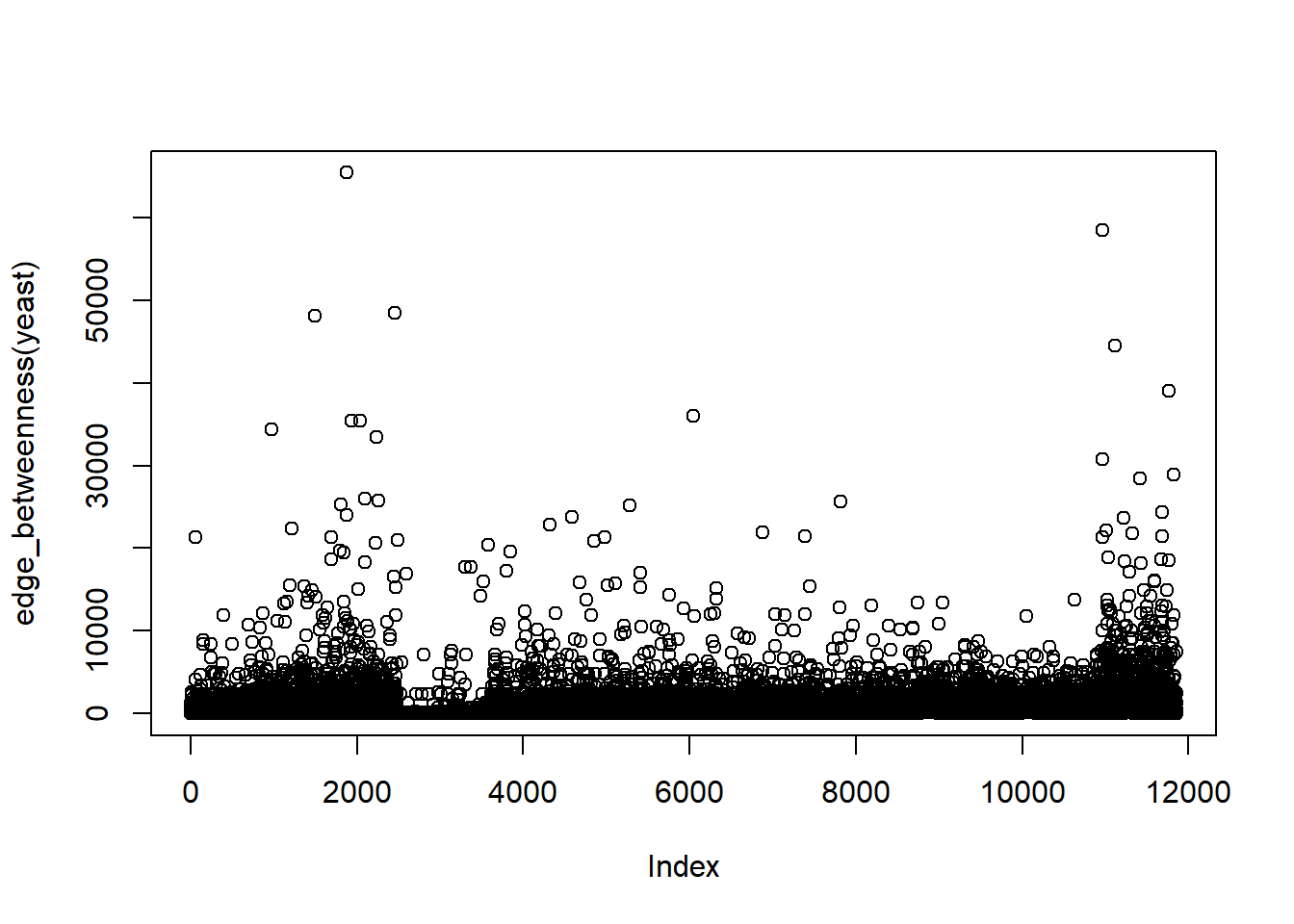
Betweenness centrality : \(C_{i}=\sum_{i\nshortparallel j\nshortparallel k}\frac{S_{j,k}(i)}{S_{j,k}}\), where \(S_{j,k}\)is the number of shortest path passing through \(k\) and \(j\) and \(S_{j,k}(i)\) is the number of shortest path passing through \(k\) and \(j\).
We illustrate these by applying them in the yeast data set available in igraph. This data set contains the protein-protein interaction of yeasts.
YPR110C
    286
YBL056W
73 YGR173W
258 YFR043C
735 [1] 1882[1] 21The distributions of these measures are as follows :
Degree
Closeness
Edge-Betweeness
Now we look at some topological characteristics of real world networks.
Average Path length : This is \(\frac{1}{|V|(|V|-1)}\sum_{i=1}^{|V|}\sum_{j=1}^{|V|}d(i,j)\) for directed graphs. For undirected graphs we multiply this by 2.
Clustering Coefficient : \(C_{i}=\frac{2\sum_{j=1}^{j=|N_{v_{i}}|}\lambda(v_{i},v_{j})}{|N_{v_{i}}|(|N_{v_{i}}|-1)}\). The clustering coefficient essentially counts the proportion of edges connected in the neighborhood of vertex \(v_{i}\).
Clique Number : A high number of cliques indicate strong cohesion between the nodes of the network.
We illustrate these in the same yeast dataset as follows :
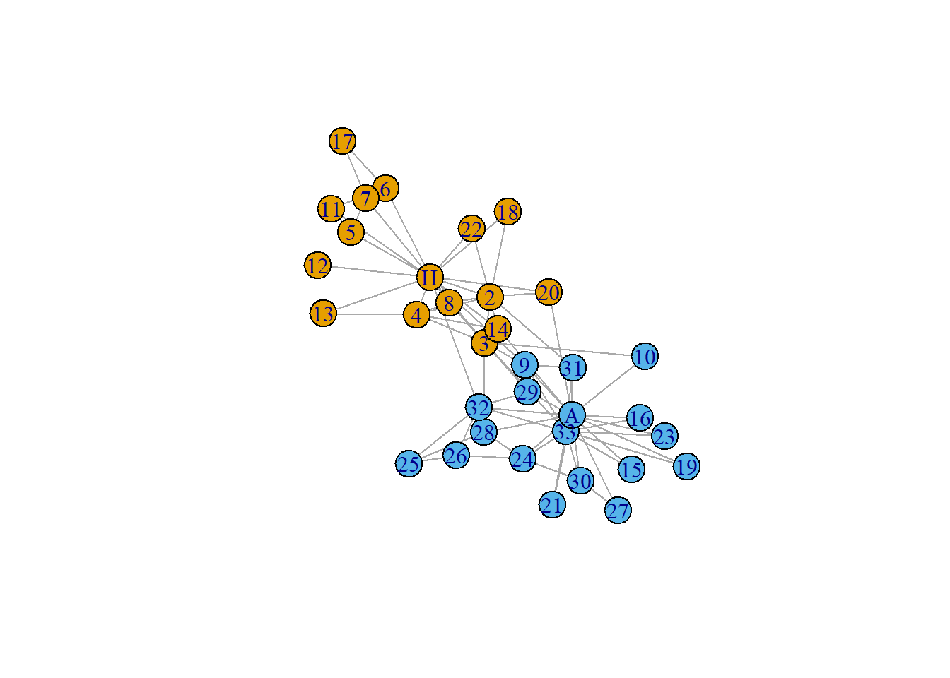
[1] 5.095629[1] 0.4686178[1] 0.0034633[1] 23Now we look at a particular dataset and analyse it. The dataset we have chosen is the Zachary Karate Club Dataset. This is a popular, classical dataset.
For any data set it is of paramount interest to understand the background of the data to perform sound analysis.
This is an example of a social network. Each link denotes a pair who interacted outside club.The details of the data set are as follows :
Social network between members of a university karate club, led by president John A. and karate instructor Mr. Hi (pseudonyms). The edge weights are the number of common activities the club members took part of. These activities were:
1. Association in and between academic classes at the university.
2. Membership in Mr. Hi\textquoteright s private karate studio on the east side of the city where Mr. Hi taught nights as a part-time instructor.
3. Membership in Mr. Hi\textquoteright s private karate studio on the east side of the city, where many of his supporters worked out on weekends.
4. Student teaching at the east-side karate studio referred to in (2). This is different from (2) in that student teachers interacted with each other, but were prohibited from interacting with their students.
5. Interaction at the university rathskeller, located in the same basement as the karate club’s workout area.
6. Interaction at a student-oriented bar located across the street from the university campus.
7. Attendance at open karate tournaments held through the area at private karate studios.
8. Attendance at intercollegiate karate tournaments held at local universities. Since both open and intercollegiate tournaments were held on Saturdays, attendance at both was impossible. Zachary studied conflict and fission in this network, as the karate club was split into two separate clubs, after long disputes between two factions of the club, one led by John A., the other by Mr. Hi. The \textquoteleft Faction\textquoteright{} vertex attribute gives the faction memberships of the actors. After the split of the club, club members chose their new clubs based on their factions, except actor no. 9, who was in John A.’ s faction but chose Mr. Hi’s club.
We note that this is an undirected weighted graph with 34 nodes.
First we plot the data :
Now we shall look into the vertex centrality measures first.
   Mr Hi  Actor 2  Actor 3  Actor 4  Actor 5  Actor 6  Actor 7  Actor 8
      16        9       10        6        3        4        4        4
 Actor 9 Actor 10 Actor 11 Actor 12 Actor 13 Actor 14 Actor 15 Actor 16
       5        2        3        1        2        5        2        2
Actor 17 Actor 18 Actor 19 Actor 20 Actor 21 Actor 22 Actor 23 Actor 24
       2        2        2        3        2        2        2        5
Actor 25 Actor 26 Actor 27 Actor 28 Actor 29 Actor 30 Actor 31 Actor 32
       3        3        2        4        3        4        4        6
Actor 33   John A
      12       17
The maximum and minimum degree(s), along with the node are respectively
John A
    34
Actor 12
12 The degree distribution is as follows :
plot(degree.distribution(karate))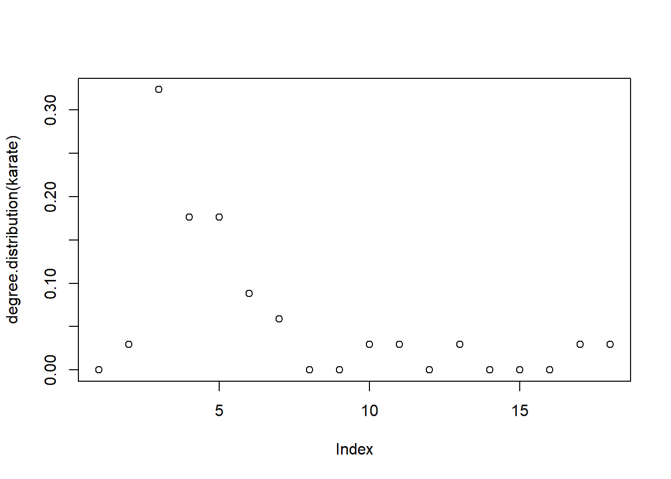
Mr Hi
    1
Actor 17
17 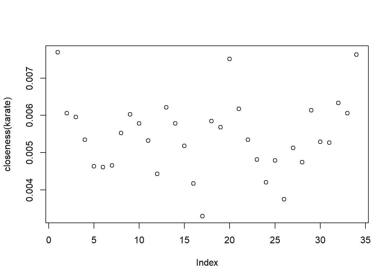
Mr Hi
    1
Actor 8
8 plot(betweenness(karate))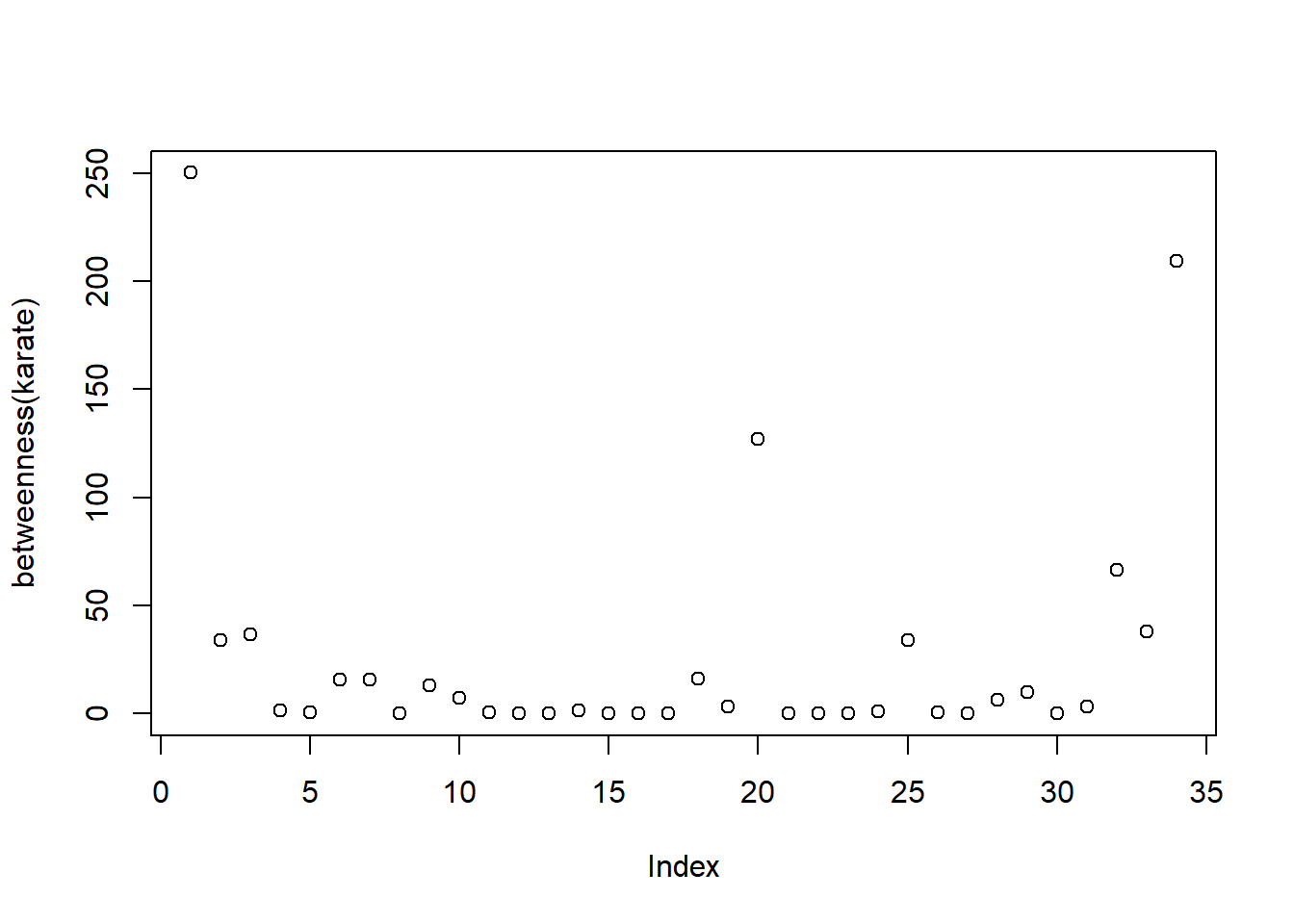
The maximum and minimum of values of edge\_betweenness, along with the node are respectively :
[1] 53[1] 1The distribution is as follows :
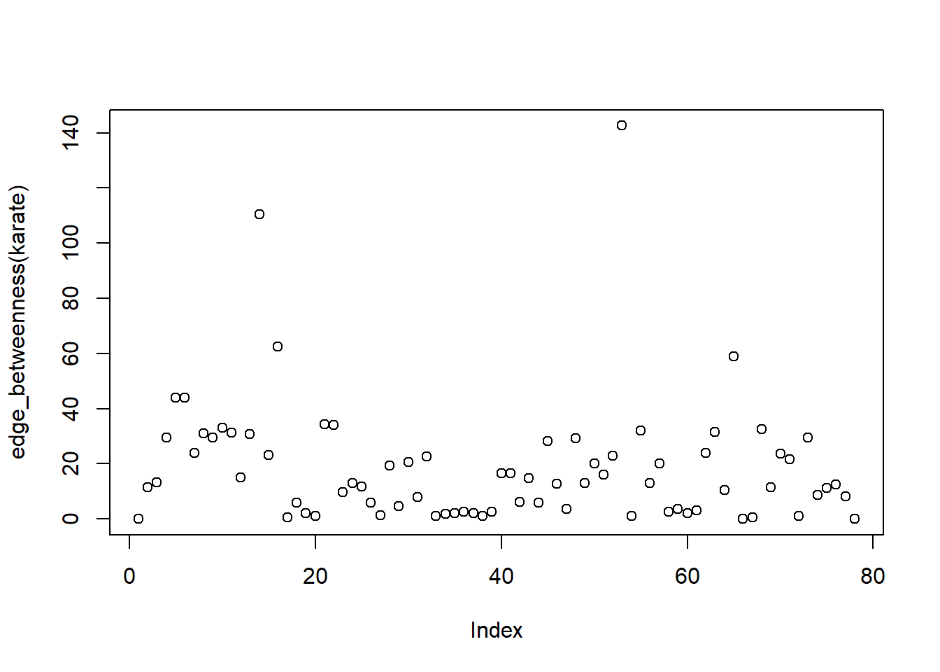
We note that all these three measures indicate that no one among the student members were particularly influential. This indicates that during the splitting of the club individual members did not play a key role and the factions depended solely on ideologies
Now we look at network cohesion measures :
Comment :
We note that the average path length is about 6. This means that on an average, any two people in the group were separated by a chain of six people. The value of APL is around 6 in real life large scale networks and such networks are called small-world network.We shall like to emphasize the point that we must also keep the size of the network in mind. Here we are only considering 34 people, and the average path length is 6. As the number of club members in consideration is so small, it sheds light on the fact that the members were not well connected outside club activities. This suggests that splitting of the club occurred mainly due to ideological differences. This fact is further supported by clustering coefficient.
[1] 0.2556818Comment :
We note that the club had low clustering coefficient. It shows that the mutual friends of an individual were not that well connected themselves. This indicates that during the splitting of the club, ``friendship between different club members’’ did not play a significant role. If the clustering coefficient was high, there was a possibility that some members chose a faction because their friends chose that faction. This provides evidence that the splitting of the club occurred based on ideological differences.
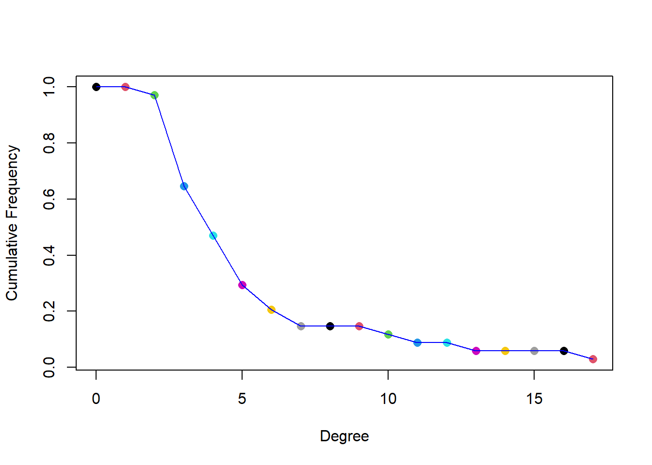
Comment :
Again we see that the proportion of people having less than 5 connections is very high ( more than \(70\%\)). This also indicates that the the members were sparsely connected.
Now we look at Community Detection based on three different algorithms.
The members of the faction(s) are as follows :
IGRAPH clustering label propagation, groups: 4, mod: 0.42
+ groups:
  $`1`
   [1] "Mr Hi"    "Actor 2"  "Actor 3"  "Actor 4"  "Actor 5"  "Actor 8"
   [7] "Actor 11" "Actor 12" "Actor 13" "Actor 14" "Actor 18" "Actor 20"
  [13] "Actor 22" "Actor 29"

  $`2`
  [1] "Actor 6"  "Actor 7"  "Actor 17"

  $`3`
   [1] "Actor 9"  "Actor 10" "Actor 15" "Actor 16" "Actor 19" "Actor 21"
+ ... omitted several groups/vertices::: {.cell}
::: {.cell-output .cell-output-stderr}
```
Warning in cluster_edge_betweenness(karate): At core/community/
edge_betweenness.c:492 : Membership vector will be selected based on the highest
modularity score.
```
:::
::: {.cell-output .cell-output-stderr}
```
Warning in cluster_edge_betweenness(karate): At core/community/
edge_betweenness.c:497 : Modularity calculation with weighted edge betweenness
community detection might not make sense -- modularity treats edge weights as
similarities while edge betwenness treats them as distances.
```
:::
::: {.cell-output-display}
{width=672}
:::
:::The members of the faction(s) are as follows :
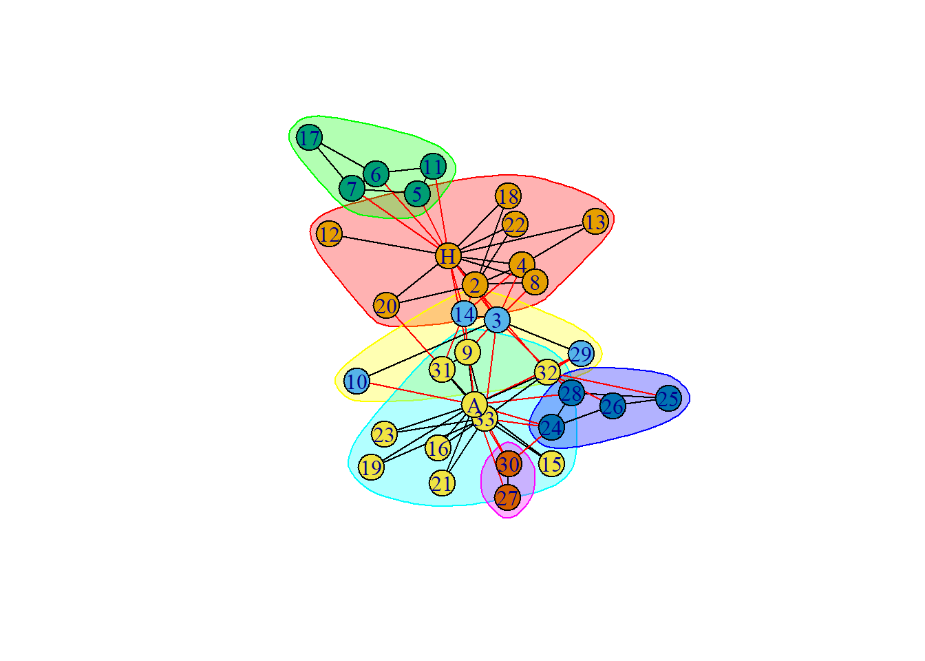
IGRAPH clustering edge betweenness, groups: 6, mod: 0.35
+ groups:
  $`1`
  [1] "Mr Hi"    "Actor 2"  "Actor 4"  "Actor 8"  "Actor 12" "Actor 13"
  [7] "Actor 18" "Actor 20" "Actor 22"

  $`2`
  [1] "Actor 3"  "Actor 10" "Actor 14" "Actor 29"

  $`3`
  [1] "Actor 5"  "Actor 6"  "Actor 7"  "Actor 11" "Actor 17"

  + ... omitted several groups/vertices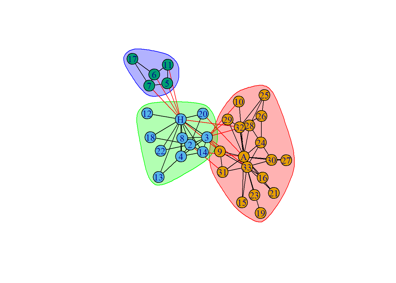
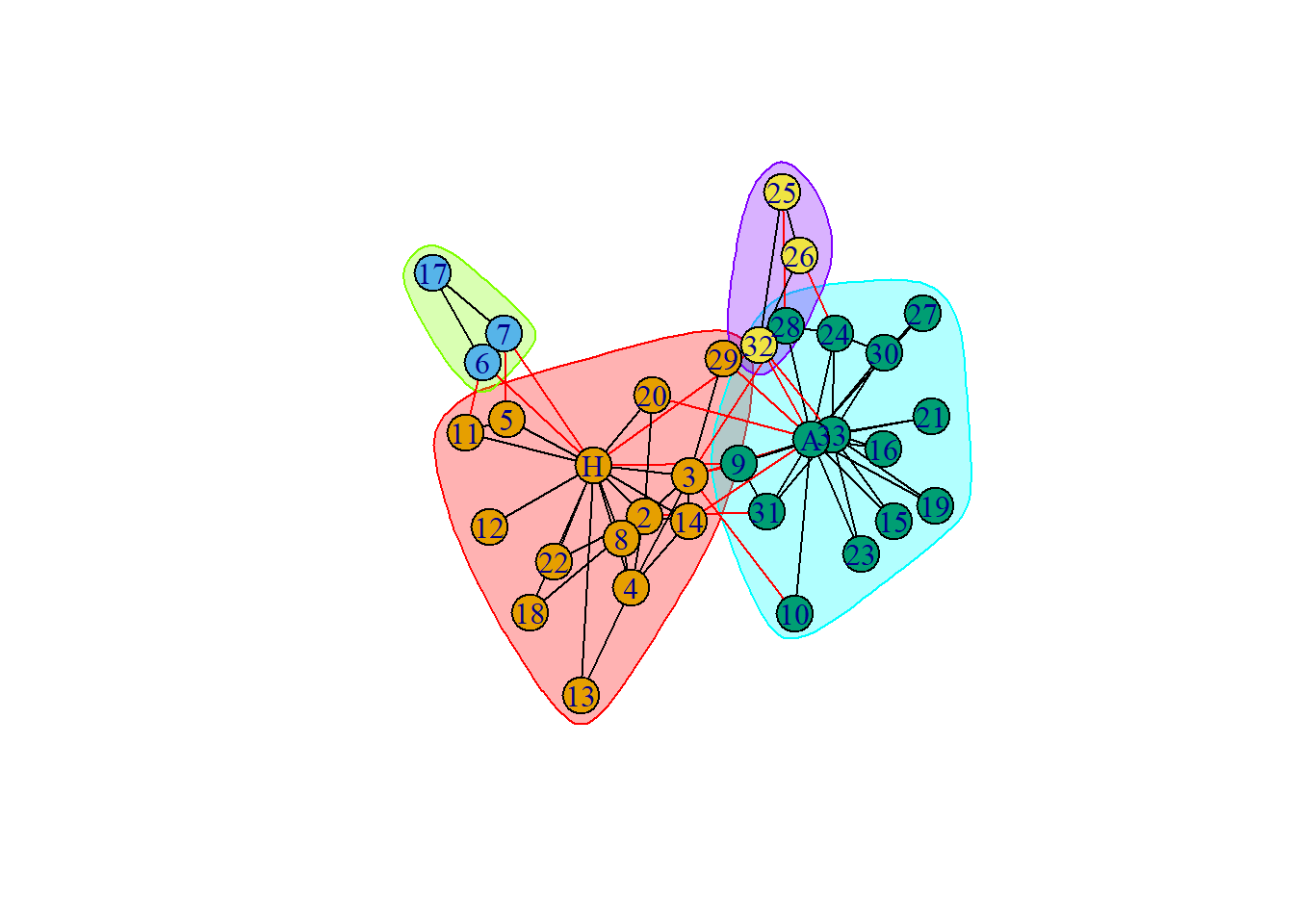
The members of the faction(s) are as follows :
IGRAPH clustering fast greedy, groups: 3, mod: 0.43
+ groups:
  $`1`
   [1] "Actor 9"  "Actor 10" "Actor 15" "Actor 16" "Actor 19" "Actor 21"
   [7] "Actor 23" "Actor 24" "Actor 25" "Actor 26" "Actor 27" "Actor 28"
  [13] "Actor 29" "Actor 30" "Actor 31" "Actor 32" "Actor 33" "John A"

  $`2`
   [1] "Mr Hi"    "Actor 2"  "Actor 3"  "Actor 4"  "Actor 8"  "Actor 12"
   [7] "Actor 13" "Actor 14" "Actor 18" "Actor 20" "Actor 22"

  $`3`
  + ... omitted several groups/vertices
We know that in reality there were two major communities. Hence, label based optimization in this case leads to better community detection, whereas edge based propagation is the worst.
This section includes supplementary material on this topic.
Graphs can be represented in the computer memory using array and list data structures. One way to store the information is by using the adjacency matrix defined before hand. Consider the adjacency matrix corresponding to the directed graph with 3 nodes plotted in the earlier section. We note that this matrix is asymmetric. Several Characteristics of the graph can be calculated using the adjacency matrix. For example :
\[deg_{i}=\sum_{j=1}^{j=n}Adj[i][j]\]
Note : Though adjacency matrices are useful, for large data sets, it might not be feasible to work with them. In these cases the list representations are used. It is stored as singly liked list where each node is listed and adjacent to each node the corresponding nodes with which it makes a pair are listed. Another advantage of using lists is that it can be used for dynamic graphs.
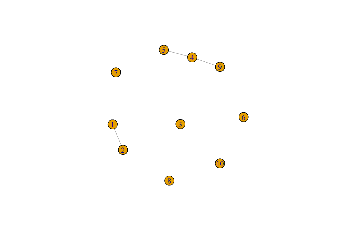
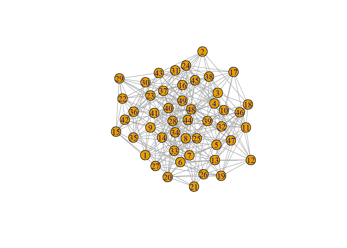
For inferential and prediction purposes, we need to model the complex real life networks. This is achieved via random graphs. Some of the popular models ( not all equally useful !) are as follows :
Generally 3 different class of graphs are defined under this model. We present a particular one. A (random) graph \(\Gamma=(V,E)\) where each pair of nodes are connected via edges with probability \(p\). Consequently the number of edges, degree of a particular node, etc are random variables. In this case the total number of edges follows $Bernoulli$ distribution. These can be simulated in R as follows :
Pietro Hiram Guzzi, Swarup Roy - Biological Network Analysis- Academic Press.
Eric D. Kolaczyk - Statistical Analysis Of Network Data-Springer.
(Use R!) Eric D. Kolaczyk, Gábor Csárdi - Statistical Analysis Of Network Data With R-Springer (2020).
Zachary’s karate club - Wikipedia.
https://sites.duke.edu/dnac/resources/datasets/.
https://rpubs.com/yanalytics/network-analysis-directed1