Introduction
When we have a random sample from some distribution, it is in our interest to approximate the cdf of our statistic by the cdf of standard normal followed by some extra terms. The Berry-Esseen theorem gives us a bound on the error of order \(O(\frac{1}{n})\) if we approximate the cdf of \(T_{n}=\frac{1}{\sqrt{n}}\sum_{i=1}^{i=n}X_{i}\) via the cdf of standard normal distribution. The question of interest is whether we can decrease the error rate by adding few (appropriate ) extra terms.Edgeworth expansion gives us exactly that. The motivation behind this result is nothing new. We know that the chf of \(T_{n}\) , \(\psi_{n}(x)=\psi^{n}(\frac{x}{\sqrt{n}})\) can be expanded using taylor series ( for complex numbers ).Here we expand via cumulants and after expanding the inversion formula is applied to obtain the result. Properties of cumulants and hermite polynomials come into play.
Suppose we have \(X_{1},X_{2},…,X_{n}\) i.i.d random variables and we are interested in approximating the probability distribution of \(T_{n}=\frac{1}{\sqrt{n}}\sum_{i=1}^{i=n}X_{i}\) ( as we generally are ). Without loss of generality we may assume that \(E[X]=0\) and \(Var[X]=1\). Now Berry Esseen’s theorem provides an approximation of order \(O(\frac{1}{\sqrt{n}})\). The question of interest is whether it is possible to obtain a better approximation. As it turns out, it is possible to obtain better approximations depending on how many cumulants exist. The result which we shall discus here is true only for statistics of the kind \(T_{n}\), though we shall see some generalizations at the end.
But, how to find such an approximation ? The idea is to use the characteristic function and approximate it by a series. Then somehow ``invert’’ that series to get an approximation of the cdf, via the inversion formula. The result is as follows :
Edgeworth Expansion : Suppose \(X_{1},X_{2},…,X_{n}\) are i.i.d random variables with mean \(0\) and variance \(1\). Suppose \(T_{n}=\frac{1}{\sqrt{n}}\sum_{i=1}^{i=n}X_{i}\). Then there exist functions \(\{p_{n}(x)\}\) and constants \(\{c_{n}\}\) such that
\[F_{n}(x)=\Phi(x)+\frac{c_{1}}{\sqrt{n}}p_{1}(x)+\frac{c_{2}}{n}p_{2}(x)+o(\frac{1}{n})\]
where \(c_{i}'s\) depend on \(cumulants\) and \(p_{i}'s\) depend on \(Hermite\) polynomials. Consequently, the order of the expansion depends on existence of cumulants.
We have not given the exact form of \(c_{i}'s\) and \(p_{i}'s\) here. We shall find them as we derive our result. However, before we begin proving the result, we must discuss some preliminary concepts, for the sake of completeness and ease of the reader.*
Inversion Formula
This is one of the most profound results in probability theory which connects the characteristic function with the cdf of a distribution. It is the following :
\[f_{X}(t)=\frac{1}{2\pi}\int e^{-itx}\psi(x)dx\]
where \(\psi(.)\) is the characteristic function. This formula will create a bridge between two results from two different concepts and help us obtain the Edgeworth expansion.
Hermite Polynomials
We know that normal distribution has some nice properties. One interesting property is that the $i^{th}$ derivative of pdf of standard normal distribution \(\phi[x]\) can be written as the prodcut of some polynomial and \(\phi(x).\)
\[\phi^{(1)}[x]=-x\phi(x)\]
\[\phi^{(2)}[x]=(x^{2}-1)\phi(x)\]
\[\phi^{(3)}[x]=-x(x^{2}-3)\phi(x)\]
\[\phi^{(4)}[x]=(x^{4}-6x^{2}+3)\phi(x)\]
\[\phi^{(5)}[x]=-x(x^{4}-10x^{2}+15)\phi(x)\]
In general, \(\phi^{(i)}[x]=H_{i}(x)\phi(x)\) , where \(H_{i}(x)\) are called Hermite Polynomials. Hence, these polynomials are defined in a recursive manner and the \(i^{th}\) Hermite polynomial can be found from \(i^{th}\)derivative of \(\phi[x]\).
An Interesting Result
Lemma : \(\frac{1}{2\pi}\int e^{-itx}e^{-\frac{t^{2}}{2}}(it)^{k}dt=(-1)^{k}H_{k}(x)\phi(x)\)
Proof :
I = \(\frac{1}{2\pi}\int e^{-itx}e^{-\frac{t^{2}}{2}}(it)^{k}dt=\frac{(-1)^{k}}{2\pi}\int_{-\infty}^{\infty}\frac{d^{k}}{dx^{k}}\{e^{-itx}\}e^{-\frac{t^{2}}{2}}dt\)
or, by interchanging the integral and differential operators we have
I \(=\frac{(-1)^{k}}{2\pi}\frac{d^{k}}{dx^{k}}\{\int_{-\infty}^{\infty}e^{-itx}e^{-\frac{t^{2}}{2}}dt\}=(-1)^{k}\frac{d^{k}}{dx^{k}}\{\phi(x)\}\) [ By applying the inversion formula ]
or,
I\(=(-1)^{k}H_{k}(x)\phi(x)\) (proved)
Cumulants
The cumulant generating function shall be denoted by $K(t)$ and it is defined as follows : \(K(t)=logE[e^{itX}]\) .
The Maclaurin expansion of \(K(t)\) gives us :
\(K(t)=\sum_{n=0}^{\infty}\frac{(it)^{n}}{n!}\kappa_{n}\) , where \(\kappa_{n}\) are the coefficients of \(\frac{t^{n}}{n!}\) in the expansion. These are called \(cumulants\). Cumulants are alternatives to moments. For two distributions moments are equal iff the cumulants are equal. We note that \(\kappa_{n}=K^{(n)}(0)\). The first few cumulants are equal to the corresponding central moments, but they deviate for $4^{th}$or higher degrees. The first few values of the cumulants are as follows :
\(\kappa_{1}=E[X]\)
\(\kappa_{2}=Var[X]\)
\(\kappa_{3}=E^{3}[X-E[X]]\)
\(\kappa_{4}=E^{4}[X-E[X]]-3Var^{2}[X]\).
We note that \(\kappa_{1}=0\) and \(\kappa_{2}=1\) if \(X\) is standardised.
\(\begin{eqnarray*} \psi(u) &=& \exp \left\{-\frac{u^2}{2}+\sum_{j\ge 3}{\frac{(iu)^j}{j!}\cdot \kappa_j}\right\} \\\Rightarrow \psi_n(u) &=& \exp \left\{-\frac{u^2}{2n}\cdot n+\sum_{j\ge 3}{\frac{(iu)^j}{j!\cdot n^{j/2}}\cdot \kappa_j\cdot n}\right\} \\&=& \exp \left\{-\frac{u^2}{2}+\frac{1}{n^{1/2}}\cdot \frac{(iu)^3\kappa_3}{3!}+\frac{1}{n}\cdot \frac{(iu)^4\kappa_4}{4!}+o\left(\frac{1}{n}\right) \right\} \\&=& e^{-\frac{u^2}{2}} \cdot \exp{ \{A\}} \quad (\texttt{say}) \\&=& e^{-\frac{u^2}{2}} \cdot \left\{1+A+\frac{A^2}{2}+\cdots\right\}\\ &=& e^{-\frac{u^2}{2}} \cdot \left\{1+\frac{1}{n^{1/2}}\cdot \frac{(iu)^3\kappa_3}{3!}+\frac{1}{n}\cdot \frac{(iu)^4\kappa_4}{4!}+\frac{1}{n}\cdot \frac{(iu)^6\kappa_3^2}{2.(3!)^2}+o\left(\frac{1}{n}\right) \right\}\\ \Rightarrow f_{n}(x)&=&\frac{1}{2\pi}\left(\int_{-\infty}^{\infty}e^{-itx}e^{-\frac{t^{2}}{2}}dt\right )+\frac{1}{2\pi}\frac{\kappa_{3}/6}{\sqrt{n}}\left(\int_{-\infty}^{\infty}e^{-itx}e^{-\frac{t^{2}}{2}}(it)^{3}dt\right )+\frac{1}{2\pi}\frac{\kappa_{4}/24}{n}\left(\int_{-\infty}^{\infty}e^{-itx}e^{-\frac{t^{2}}{2}}(it)^{4}dt\right ) \\& & +\frac{1}{2 \pi}\frac{\kappa_{3}^{2}/72}{n}\left(\int_{-\infty}^{\infty}e^{-itx}e^{-\frac{t^{2}}{2}}(it)^{6}dt\right )+o\left(\frac{1}{n}\right ) \\&=&\phi(x)\left\{1+\frac{(-1)^3\cdot \kappa_{3}/6}{\sqrt{n}}H_{3}(x)+\frac{(-1)^4\cdot \kappa_{4}/24}{n}H_{4}(x)+\frac{(-1)^6\cdot \kappa_{3}^{2}/72}{n}H_{6}(x)+o\left(\frac{1}{n}\right )\right\} \\&=&\phi(x)+\frac{(-1)^3\cdot \kappa_{3}/6}{\sqrt{n}}H_{3}(x)\phi(x)+\frac{(-1)^4\cdot \kappa_{4}/24}{n}H_{4}(x)\phi(x)+\frac{(-1)^6\cdot \kappa_{3}^{2}/72}{n}H_{6}(x)\phi(x)+o\left(\frac{1}{n}\right ) \\\end{eqnarray*}\)
Now, by calculating the antiderivatives, we have :
\(F_{n}(x)=\Phi(x)+\left\{-\frac{\kappa_{3}/6}{\sqrt{n}}H_{2}(x)\phi(x)+\frac{\kappa_{4}/24}{n}H_{3}(x)\phi(x)+\frac{\kappa_{3}^{2}/72}{n}H_{5}(x)\phi(x)+o\left(\frac{1}{n}\right)\right \}\)
Therefore, the \(1^{st}\) and \(2^{nd}\) Edgeworth expansions are as follows :
$\(F_{n}(x)=\Phi(x)-\frac{\kappa_{3}/6}{\sqrt{n}}(x^{2}-1)\phi(x)\)
\(F_{n}(x)=\Phi(x)-\frac{\kappa_{3}/6}{\sqrt{n}}(x^{2}-1)\phi(x)-\frac{\kappa_{4}/24}{n}(x^{3}-3x)\phi(x)-\frac{\kappa_{3}^{2}/72}{n}(x^{5}-10x^{3}+15x)\phi(x)\)
Some important points about Edgeworth Expansions
If the underlying distribution F has moments of all orders, one is tempted to let \(k\) to \(\infty\) for better approximation. Unfortunately, the resulting infinite series need not converge for any n.
In fact Cramer showed that this series converges for all n if and only if \(e^{\frac{x^2}{4}}\) is integrable with respect to \(F\).
When the asymptotic distribution is not normal, similar expansions may be obtained by proper Taylor expansion
The approximation provided by the Edgeworth expansion is in general reliable in the center of the distribution for moderate sample sizes.
Unfortunately, the approximation deteriorates in the tails where it can even become negative.
Moreover, the absolute error is uniformly bounded over the whole range of the distribution, but the relative error is in general unbounded
A More General Result
We have derived the edgeworth expansion only for statistics of a particular kind. Then why stop there ? Can we not do somthing similar for other kind of statistics ? Note that we have exploited the particular form of the characteristic function obtained due the \(T_{n}\). Not all statistics are simply summations of \(X_{i}'s\). However, there are several important statistics which can be written as as sum of some function of \(X_{i}'s\) divided by some function of \(n\) , the sample size. Most of these come under the category of \(U-statistics\). There are some generalisations of Edgeworth expansions for U-statistics.We state that as follows :
Theorem ( Bicket 1986) : Suppose we have U-statistics of degree 2, \(U_{n}=\frac{1}{C(n,2)}\sum h(X_{i},X_{j})\). Let \(F_{n}(x)=P(\frac{U_{n}}{\sigma_{n}}<x)\). Under some conditions, there exist constants \(\lambda_{n}'s\) such that :
\(F_{n}(x)=\Phi(x)+\frac{\lambda_{1}/6}{\sqrt{n}}(x^{2}-1)\phi(x)+\frac{\lambda_{2}/24}{n}(-x^{3}+3x)\phi(x)+\frac{\lambda_{3}/72}{n}(-x^{5}+10x^{3}-15x)\phi(x)+o(\frac{1}{n})\)
The conditions are :
\(E(|h(X_{1},X_{2})|^{r})<\infty\) where \(r>2\) is a real number and \(k\) is an integer such that \((r-2)(k-4)>8\)
\(E(|h_{1}(X_{1})|^{4})<\infty\)
\(limsup_{|x|->\infty}|E(e^{ixh_{1}(X)}<1|\)
\(|\lambda_{i}|\)’s are eigen values of kernel \(h.\) That is : \(\int h(x_{1},x_{2})w_{j}(x_{1})dF(x_{1})=\lambda_{j}w_{j}(x_{2})\),
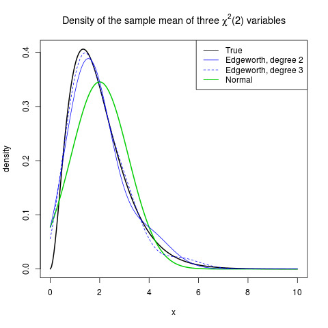
Illustration with an Example
Suppose \(X_{1},X_{2},X_{3}\sim\chi(2).\) Then the sample mean follows \(\Gamma(3,\frac{2}{3}).\)Now we can plot the actual distribution, Edgeworth expansions of order \(2\) and \(3\) , as well as the limiting distribution of the sample mean. We plot these \(4\) and see what happens ( courtesy Wikipedia ).