install.packages("devtools")Introduction
This package is created jointly with my friend Mainak Manna. This is a result of our project on density estimation as a part our coursework on Nonparametric Inference. This package consists of 19 functions as of now. It is live and currently uploaded on my GitHub account. I shall first discuss how to install and use our package and then show some examples. I encourage others to use it and let us know of any mistakes or problems which they face.
How to use densest
It is very simple to install and use this package. There is no need to go to my GitHub account to access it. One can easily install and use it directly in RStudio. The steps are as follows ( you might copy these directly to clipboard ) :
Install the package “devtools”
Now we can use the function “install_github” in place of “install.packages”. The code snippet required is given below
install_github("SPRstat/Density-Estimation-R-Package-")After the package is installed, load it like any other package.
library(densest)
That is all. Now you are all set !
Using Help Files
Every function in this package has a help file. To access the help files, use the same commands as in regular functions.
?MISE()You will see a documentation like the one below.
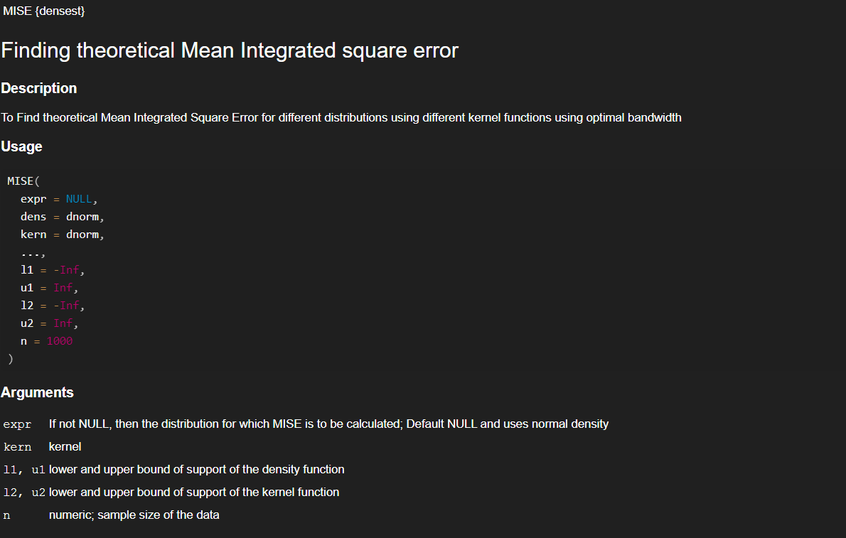
About the package
The package can be used to study theoretical properties of several methods of density estimation. The package currently has 19 functions. Some of them are quite useful, while some others might not be very relevant for everyone. We shall mention some important functions in this section.
beta_density( )
All of you must have observed that by varying the values of the two parameters of the beta distribution, one can obtain almost all kind of shapes “generally” exhibited by “well behaved” probability density functions, on support \((0,1)\) . Now, suppose we have observations \(X_1,X_2,...,X_n\) . We transform these random variables to \((0,1)\) by applying \(X_i\) \(-\) \(X_(1)\) / \(Range\) . Then find MOM estimates of the parameters and obtain a “beta-density” estimate. Then apply suitable inverse transformation to obtain the density estimate on the original support. An illustration with usage in R exhibiting performance is as follows :
par(mfrow = c(3,3))

curve(dnorm(x),-3,3,xlab = "N(0,1)",type = "l",col = "blue")
curve(beta_density(x,rnorm(1000)),-3,3,xlab = "N(0,1)",ylab="",add = TRUE,col = "red")

curve(dcauchy(x),-30,30,xlab = "C(0,1)",type = "l",col = "blue")
curve(beta_density(x,rcauchy(1000)),-30,30,xlab = "C(0,1)",ylab="",add = TRUE,col = "red")

curve(dchisq(x,df = 5),0,30,xlab = "Chi(5)",type = "l",col = "blue")
curve(beta_density(x,rchisq(1000,df = 5)),0,30,xlab = "Chi(5)",ylab="",add = TRUE,col = "red")

curve(dexp(x),0,5,xlab = "Exp(1)",type = "l",col = "blue")
curve(beta_density(x,rexp(1000)),0,5,xlab = "Exp(1)",ylab="",add = TRUE,col = "red")

curve(dlogis(x),-10,10,xlab = "S.Logis",type = "l",col = "blue")
curve(beta_density(x,rlogis(1000)),-10,10,xlab = "S.Logis",ylab="",add = TRUE,col = "red")

curve(dunif(x),0,1,xlab = "Uni(-1,1)",type = "l",col = "blue")
curve(beta_density(x,runif(1000)),0,1,xlab = "Uni(-1,1)",ylab="",add = TRUE,col = "red")

curve(dweibull(x,5),0,10,xlab = "Wei(5)",type = "l",col = "blue")
curve(beta_density(x,rweibull(1000,5)),0,10,xlab = "Wei(5)",ylab="",add = TRUE,col = "red")

curve(dt(x,5),-3,3,xlab = "t(5)",type = "l",col = "blue")
curve(beta_density(x,rt(1000,df = 5)),-3,3,xlab = "t(5)",ylab="",add = TRUE,col = "red")

curve(dt(x,3,4),0,15,xlab = "F(3,4)",type = "l",col = "blue")
curve(beta_density(x,rf(1000,3,4)),0,15,xlab = "F(3,4)",ylab="",add = TRUE,col = "red")
mtext("Beta Estimates for data from different (Cont) Distributions",side=3,outer=TRUE,padj=3)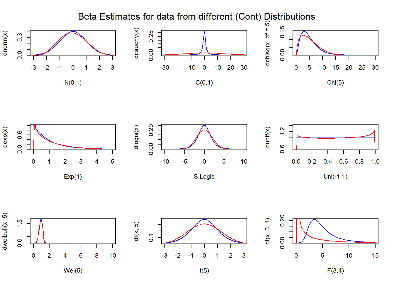
kern_density( )
Using this function one can obtain density estimates using the method of kernel density estimation. One can choose different kernels like the “naive kernel”, “triangular kernel”, “normal kernel” and “optimal kernel”. One has to input the vector of observations, choice of kernel and bandwidth. For illustration we simulate two set of observations, one from standard normal and another from \(Chi(5)\) .
- Chi-Square(5)
par(mfrow = c(2,2))
f.chisq = function(n){dchisq(n,df=5)}
curve(kern_density(x,vec.chisq,func=naive_kern,h=.6),0,10,ylab="naive",col = "red")
curve(f.chisq,0,10,add = TRUE,lty = 3,lwd = 2)
curve(kern_density(x,vec.chisq,func=dnorm,h=.6),0,10,ylab="norm",col = "blue")
curve(f.chisq,0,10,add = TRUE,lty = 3,lwd = 2)
curve(kern_density(x,vec.chisq,func=triangular_kern,h=.6),0,10,ylab="triangular",col = "green")
curve(f.chisq,0,10,add = TRUE,lty = 3,lwd = 2)
curve(kern_density(x,vec.chisq,func=opt_kern,h=.6),0,10,ylab="optimal",col = "brown")
curve(f.chisq,0,10,add = TRUE,lty = 3,lwd = 2)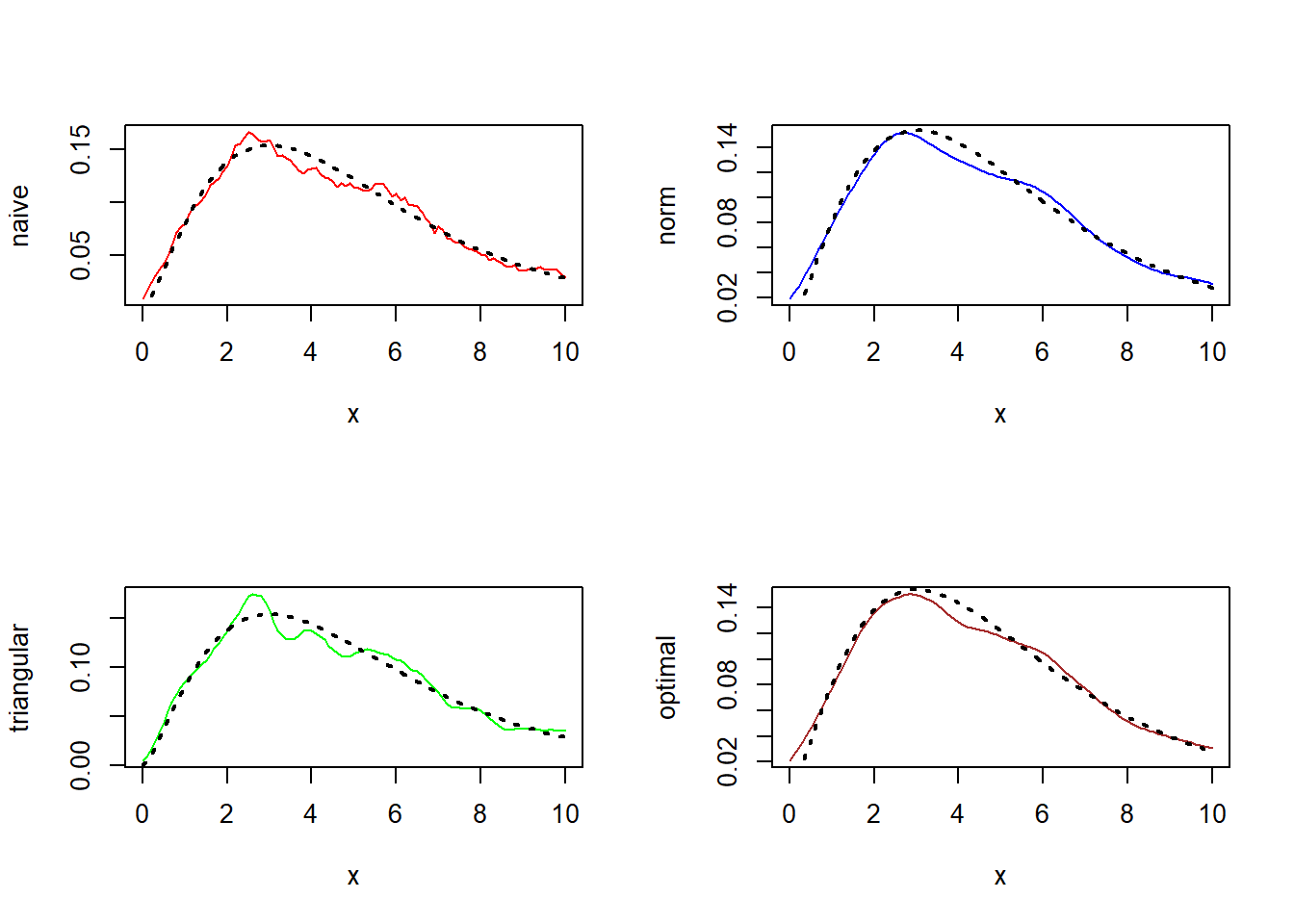
Standard Normal
par(mfrow = c(1,1))
curve(kern_density(x,vec,func=naive_kern,h=.46),-3,3,ylab = "",col = "red",lwd=2)
curve(kern_density(x,vec,func=dnorm,h=.26),-3,3,ylab="norm",add = TRUE,col = "blue",lwd=2)
curve(kern_density(x,vec,func=triangular_kern,h=.64),-3,3,ylab="triangular",add = TRUE,col = "green",lwd=2)
curve(kern_density(x,vec,func=opt_kern,h=.26),-3,3,ylab="optimal",add = TRUE,col = "brown",lwd=2)
legend(x = "topright",legend = c("Naive","Norm","Triangular","Optimal"),col = c("red","blue","green","brown"),lwd = 2)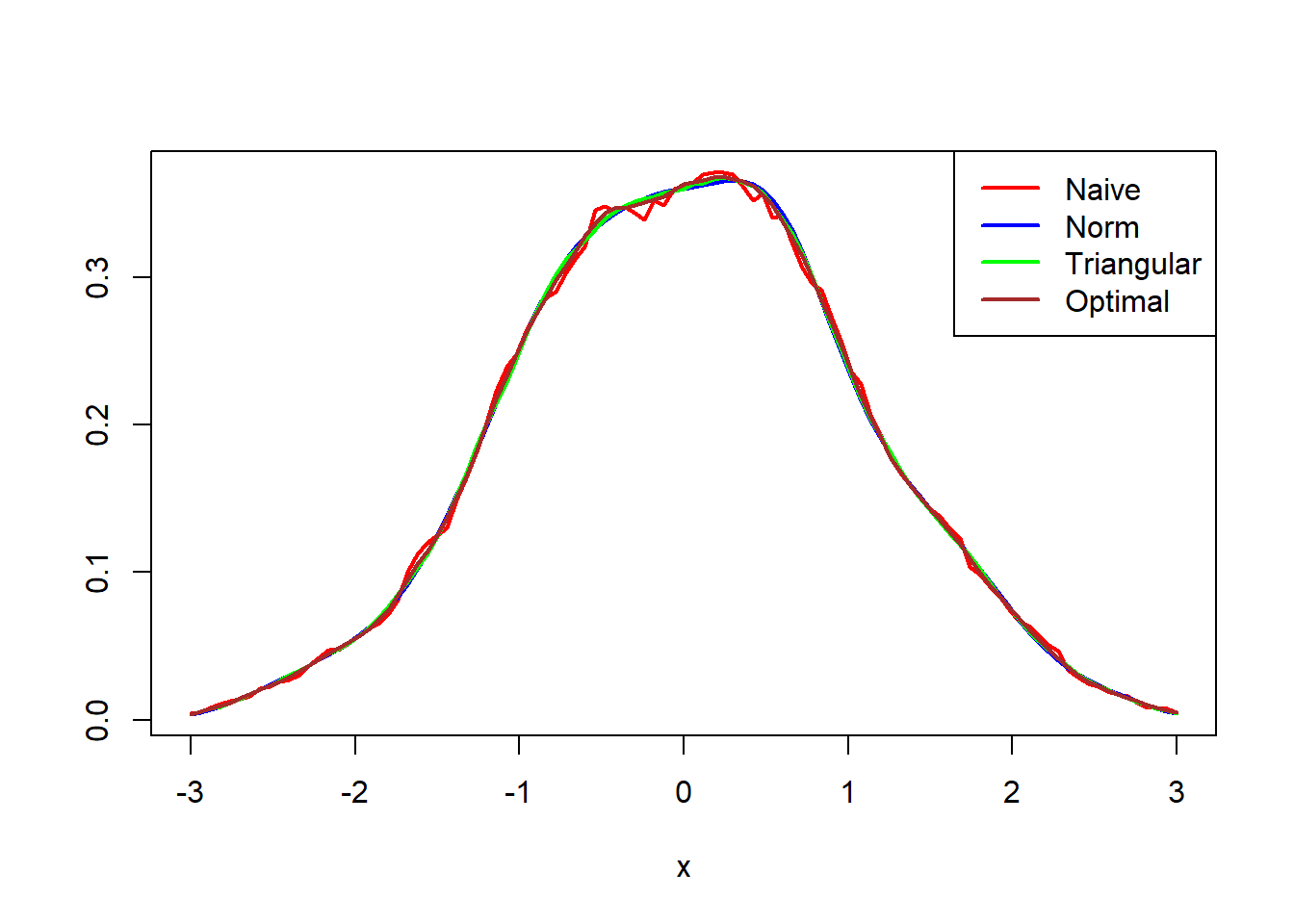
MISE( )
This is one of the most important functions in our package. While studying different kernel density estimates one might be interested to find the value of actual theoretical value of MISE. One might also be interested to find the value of optimal bandwidth for their research (or application). This function does both. One can find optimal bandwidth and theoretical value of MISE by varying underlying distribution, as well as the kernel. There are two additional functions with same utility, but targeted for bias reduction using kernels which can take negative values, as well as distributions with restrictions on the support. An illustration of MISE function is as follows :
Calculating theoretical MISE for different underlying distribution and Kernels
under_dist=c(normal_exp(),cauchy_exp(),logis_exp())
kernel_density_es=c(dnorm,naive_kern,triangular_kern,opt_kern)
l_limit=c(-Inf,-Inf,-100)
u_limit=c(Inf,Inf,100)
n_d=seq_along(under_dist)
n_k=seq_along(kernel_density_es)
d=expand.grid(n_d,n_k)
optimal_bw=apply(d, 1, function(x){MISE(expr=as.expression(under_dist[[x[1]]]),kern=kernel_density_es[[x[2]]],l1=l_limit[x[1]],u1=u_limit[x[1]])$h_opt})
optimal_bw=matrix(optimal_bw,nrow = length(n_d),byrow = FALSE)
colnames(optimal_bw)=c("normal krenel","naive kernel","triangular kernel","otimal kernel")
rownames(optimal_bw)=c("normal density","cauchy density","logistic density")
optimal_mise=apply(d, 1, function(x){MISE(expr=as.expression(under_dist[[x[1]]]),kern=kernel_density_es[[x[2]]],l1=l_limit[x[1]],u1=u_limit[x[1]])$mise})
optimal_mise=matrix(optimal_mise,nrow = length(n_d),byrow = FALSE)
colnames(optimal_mise)=c("normal krenel","naive kernel","triangular kernel","otimal kernel")
rownames(optimal_mise)=c("normal density","cauchy density","logistic density")
optimal_bw
normal krenel naive kernel triangular kernel otimal kernel
normal density 0.2660650 0.4629683 0.6470696 0.2634150
cauchy density 0.1642997 0.2858909 0.3995766 0.1626633
logistic density 0.4118403 0.7166257 1.0015949 0.4077383Concluding Remarks
This post is meant to be an introduction to our package. We have only discussed three functions in this post. However, there are several other useful functions as well. There are functions which can for example approximate MISE for \(L_1\) loss function using Monte Carlo simulation, or calculate Integrated Square Error, etcetera. We encourage the readers to explore the help files for more exposure to our package.